
| 일 | 월 | 화 | 수 | 목 | 금 | 토 |
|---|---|---|---|---|---|---|
| 1 | 2 | 3 | ||||
| 4 | 5 | 6 | 7 | 8 | 9 | 10 |
| 11 | 12 | 13 | 14 | 15 | 16 | 17 |
| 18 | 19 | 20 | 21 | 22 | 23 | 24 |
| 25 | 26 | 27 | 28 | 29 | 30 | 31 |
- Yeo-Johnsom 변환
- 데이터 분석
- FWER
- cltv
- python significance level
- 베이지안론
- error bar plot
- 데이터 시각화
- 시각화
- 분위수 변환
- python error plot
- matplotlib
- box-cox변환
- spearman
- ecommerce data
- 고객가치분석
- data analysis
- p value plot
- 백분위 변환
- ttest
- E-Commerce
- 통계
- Pearson
- plot
- marketing insight
- 빈도주의론
- marketing
- lifetimevalue
- 다중검정
- python
- Today
- Total
Data 공부
BTS의 성공요인 분석 - 토픽모델링과 소셜 네트워크 분석 활용 본문
BTS의 성공요인 분석 - 토픽모델링과 소셜 네트워크 분석 활용
* 졸업논문 프로젝트를 정리하여 작성
상대적으로 약자에서 시작했지만, 언더독(Underdog)의 열정을 통해 역경을 극복한 스토리는 많은 사람들에게 감동과 희망을 전달하고 2, 3차의 연쇄적 긍정 효과를 가져옵니다. 방탄소년단(BTS)는 대표적인 언더독 스토리의 주인공으로 한국 최초 빌보드 1위 기록과 함께 전 세계적인 팬덤을 구축했으며, 영향력이 커지고 있습니다.
방탄소년단은 중소기획사 출신으로서 가지는 제약을 극복하고자 트위터, 유튜브 등의 소셜미디어를 데뷔 초부터 적극 활용하여 다양한 콘텐츠를 공유하였으며, 적극적으로 팬들과 소통하였습니다.

목표 :
이에 아이디어를 얻어 소셜미디어 데이터를 이용하여 BTS의 성공요인을 분석해봅니다.
1. 변곡점 선정 ( LDA, 소셜네트워크 분석은 변곡점의 기간에 맞춰 분석)
2. twitter crawling / 시계열 자료 수집
3. 데이터 가공
4. LDA (Latent Dirichlet Allocation)
5. 소셜네트워크 분석
6. 결과해석
7. 결론 및 한계점
1. 변곡점 선정
BTS의 인기 변곡점을 2가지로 설정하였다.
1) 2015년 4월 -<화양연화 pt.1> 발매 및 데뷔 이후 첫 1위
2) 2017년 11월 - 'AMAs' 무대로 첫 미국 데뷔
2-1. 시계열 자료

2-2. twitter 데이터 수집
Firefox와 selenium을 이용하여 'BTS' 키워드가 들어간 영어 tweet 크롤링 (2014년 1월 - 2020년 12월)
|
1
2
3
4
5
6
7
8
9
10
11
12
13
14
15
16
17
18
19
20
21
22
23
24
25
26
27
28
29
30
31
32
33
34
35
36
37
38
39
40
41
42
43
44
45
46
47
48
49
50
51
52
53
54
55
56
57
58
59
60
61
62
63
64
65
66
67
68
69
70
71
72
73
74
75
76
77
78
79
80
81
82
83
84
85
86
87
88
89
|
#firefox 와 selenium을 이용하여 'BTS' 키워드가 들어간 영어 tweet 크롤링
from bs4 import BeautifulSoup
import requests
from selenium import webdriver
from selenium.webdriver.firefox.firefox_binary import FirefoxBinary
from selenium.webdriver.common.desired_capabilities import DesiredCapabilities
import time
from selenium.webdriver.common.keys import Keys
import datetime as dt
import pandas as pd
binary = FirefoxBinary('C:/Program Files/Mozilla Firefox/firefox.exe')
browser = webdriver.Firefox(executable_path='C:/Program Files/Mozilla Firefox/geckodriver.exe', firefox_binary=binary)
startdate = dt.date(year=2014, month=1, day=1) #tweeter는 한번에 30일 이상 크롤링하면 중단되는 현상이 나와 한달단위 크롤링
untildate = dt.date(year=2014, month=1, day=2)
enddate = dt.date(year=2014, month=1, day=30)
tweet_list1 = []
id_list1= []
date_list1 = []
while not enddate == startdate: #startedate ~ enddate까지 crawling
url = 'https://twitter.com/search?q=BTS lang:en%20since%3A' + str(startdate) + '%20until%3A' + str(untildate) + '&amp;amp;amp;amp;amp;lang=eg' # BTS를 검색하여 나오는 tweet 추출
browser.get(url)
html = browser.page_source
soup = BeautifulSoup(html, 'html.parser')
lastHeight = browser.execute_script("return document.body.scrollHeight") # 스크롤다운
while True:
# tweet id, tweet 내용, tweet 시간에 맞는 class 선택
ids = soup.find_all("div", {"class": "css-901oao css-bfa6kz r-18jsvk2 r-1qd0xha r-a023e6 r-b88u0q r-rjixqe r-bcqeeo r-1udh08x r-3s2u2q r-qvutc0"})
tweets = soup.find_all("div", {"class": "css-901oao css-16my406 r-poiln3 r-bcqeeo r-qvutc0"})
dates = soup.find_all("a",{"class":"css-4rbku5 css-18t94o4 css-901oao r-m0bqgq r-1loqt21 r-1q142lx r-1qd0xha r-a023e6 r-16dba41 r-rjixqe r-bcqeeo r-3s2u2q r-qvutc0"})
browser.execute_script("window.scrollTo(0, document.body.scrollHeight);")
time.sleep(1)
newHeight = browser.execute_script("return document.body.scrollHeight")
if newHeight != lastHeight:
html = browser.page_source
soup = BeautifulSoup(html, 'html.parser')
ids = soup.find_all("div", {"class": "css-901oao css-bfa6kz r-18jsvk2 r-1qd0xha r-a023e6 r-b88u0q r-rjixqe r-bcqeeo r-1udh08x r-3s2u2q r-qvutc0"})
tweets = soup.find_all("div", {"class": "css-901oao r-18jsvk2 r-1qd0xha r-a023e6 r-16dba41 r-rjixqe r-bcqeeo r-bnwqim r-qvutc0"})
dates = soup.find_all("a",{"class":"css-4rbku5 css-18t94o4 css-901oao r-m0bqgq r-1loqt21 r-1q142lx r-1qd0xha r-a023e6 r-16dba41 r-rjixqe r-bcqeeo r-3s2u2q r-qvutc0"})
wordfreq = len(tweets)
for text in tweets:
tweet_list1.append(text.text)
for id in ids:
id_list1.append(id.text)
for date in dates:
date_list1.append(date.text)
else:
startdate = untildate
untildate += dt.timedelta(days=1) # untildate + 1 (date형태로)
break
lastHeight = newHeight
from pandas import DataFrame
import re
# crawling 내용 csv로 저장
pd.set_option('display.max_row', 500)
pd.set_option('display.max_columns', 100)
df = pd.DataFrame([x for x in zip(date_list1,id_list1,tweet_list1)])
df.columns=["date","id","tweet"]
#2014년1월1일 -> 2014.1.1
df['date'] = df['date'].map(lambda x: re.sub(r'년', '.', x))
df['date'] = df['date'].map(lambda x: re.sub(r'월', '.', x))
df['date'] = df['date'].map(lambda x: re.sub(r'일', '.', x))
def claer_latin1_hex_chars(text): #latin hex 언어 지우기
text = re.sub(r'(||x(.){2})','',text)
return text
df['id']=df['id'].apply(claer_latin1_hex_chars)
df['tweet']=df['tweet'].apply(claer_latin1_hex_chars)
df.to_csv('BTS크롤링 2014_1월.csv', index=False)
|
cs |
3. 데이터 가공
1) 소문자변환 및 특수문자제거
2) tweet data 중 keyword만 추출
3) 불용어제거, 표제어추출, 너무 짧거나 긴 단어 제거
4) LDA 및 소셜네트워크 분석에 사용할 corpus와 texts 생성
|
1
2
3
4
5
6
7
8
9
10
11
12
13
14
15
16
17
18
19
20
21
22
23
24
25
26
27
28
29
30
31
32
33
34
35
36
37
38
39
40
41
42
43
44
45
46
47
48
49
50
51
52
53
54
55
56
57
58
59
60
61
62
63
64
65
66
67
68
69
70
71
72
73
74
75
76
77
78
79
80
81
82
83
84
85
86
87
88
89
90
91
92
93
94
95
96
97
98
99
100
101
102
103
104
105
106
107
108
109
|
import glob
import pandas as pd
import warnings
warnings.filterwarnings("ignore", category = DeprecationWarning) # warning 무시
input_file = r'C:/Users/xodus/junseok/bts' #경로
allFile_list = glob.glob(os.path.join(input_file, 'BTS*')) # glob함수로 BTS로 시작하는 파일들을 모은다
allData = []
for file in allFile_list:
df = pd.read_csv(file)
allData.append(df)
data = pd.concat(allData, axis =0, ignore_index = True)
tweet = list(np.array(data['tweet'].tolist())) # tweet,date,id 중 tweet 부분만 추출
os.environ['MALLET_HOME'] = 'C:/Users/xodus/Downloads/mallet-2.0.8/mallet-2.0.8' # gensim모델 사용하기 위한 mallet 환경변수 선언
def preprocess_text(text): #전처리 함수
# 분석을 위해 text를 모두 소문자로 변환합니다.
text = text.lower()
# @와 #을 제외한 특수문자로 이루어진 문자열 symbols를 만듭니다.
symbols = punctuation.replace('@', '').replace('#', '')
# symbols 변수를 이용해 text에서 @와 #을 제외한 모든 특수문자를 제거합니다.
for sb in symbols :
text = text.replace(sb, '')
# text를 공백을 기준으로 구분합니다.
words = text.split()
return words
for i in range(len(tweet)):
tweet[i] = preprocess_text(tweet[i])
# 트위터 멘션, 해쉬태그, 키워드 분류
keyword, hashtag, mention = [], [], []
for word in tweet:
keyword, hashtag, mention = [], [], []
for i in range(len(word)):
if word[i][0]=='#' :
hashtag.append(word[i]) # '#'로 시작할 경우 해쉬태그
if word[i][0]=='@' :
mention.append(word[i]) # '@'로 시작할 경우 멘션
if (word[i][0]!='#' and word[i][0]!='@') : # 나머지는 keyword
keyword.append(word[i])
hashtags.append(hashtag)
mentions.append(mention)
keywords.append(keyword)
tweet = pd.DataFrame([x for x in zip(keywords,hashtags,mentions)])
tweet.columns=["keywords","hashtags","mentions"]
from nltk.corpus import stopwords
from nltk.stem import WordNetLemmatizer
stop = stopwords.words('english')
# 기존의 nltk에서 제공하는 stopwords에 지정한 stopwords 추가
stop.extend(['july','february','march','april','may','june','august','september','october','november','december','january','tomorrow','morning','time',
'tuesday','monday','thursday','wednesday','friday','saturday','sunday','today','yesterday','day','tonight','night','date','day','week'])
# 불용어 제거
tweet['keywords'] = tweet['keywords'].apply(lambda x: [word for word in x if word not in (stop)])
# 표제어 추출 (3인칭 단수 => 1인칭 , 과거 현재형 동사를 현재형으로)
from nltk.stem import WordNetLemmatizer
tweet['keywords'] = tweet['keywords'].apply(lambda x : [WordNetLemmatizer().lemmatize(word, pos='v') for word in x])
# 길이가 3 이하, 15이상인 단어는 제거
tokenized_doc1 = tweet['keywords'].apply(lambda x : [word for word in x if len(word) > 3 ])
tokenized_doc = tokenized_doc1.apply(lambda x : [word for word in x if len(word) < 15 ])
data_words = list(tokenized_doc)
def make_bigrams(texts): # 예를들어 little,boy -> little_boy
return [bigram_mod[doc] for doc in texts]
def lemmatization(texts, allowed_postags = ['NOUN']): # 어간추출 (명사만 추출하는 함수)
texts_out = []
nlp = spacy.load('en_core_web_sm', disable=['parser','ner'])
for sent in texts:
doc = nlp(" ".join(sent))
texts_out.append([token.lemma_ for token in doc if token.pos_ in allowed_postags])
return texts_out
data_words_bigrams = make_bigrams(data_words) # bigram 생성
data_lemmatized = lemmatization(data_words_bigrams, allowed_postags=['NOUN']) # data에서 명사만 추출
id2word = corpora.Dictionary(data_lemmatized) # 정수 인코딩과 빈도수 생성
texts = data_lemmatized # 명사만 추출한 data
corpus = [id2word.doc2bow(text) for text in texts] # id2word를 통해 생성한 corpus
|
cs |
4. LDA를 통한 토픽모델링
1) LDA model 생성 및 coherence_value를 이용하여 최적의 num_topic 찾기
|
1
2
3
4
5
6
7
8
9
10
11
12
13
14
15
16
17
18
19
20
21
22
23
24
25
26
27
28
29
30
31
32
33
34
35
36
|
from gensim.models.wrappers import LdaMallet
from gensim.models import CoherenceModel
import pyLDAvis
import pyLDAvis.gensim
import matplotlib.pyplot as plt
mallet_path = 'C:/Users/xodus/Downloads/mallet-2.0.8/mallet-2.0.8/bin/mallet'
# lda model 생성
ldamallet = gensim.models.wrappers.LdaMallet(mallet_path, corpus = corpus , num_topics = 20, id2word = id2word)
# coherence_value를 이용하여 최적의 num_topic찾는 함수
def compute_coherence_values(dictionary, corpus, texts, limit, start=5, step=3):
coherence_values =[]
model_list = []
for num_topics in range(start, limit, step):
model = gensim.models.wrappers.LdaMallet(mallet_path, corpus=corpus, num_topics=num_topics, id2word=id2word)
model_list.append(model)
coherencemodel = CoherenceModel(model=model, texts=texts, dictionary=dictionary, coherence='c_v')
coherence_values.append(coherencemodel.get_coherence())
return model_list, coherence_values
model_list, coherence_values = compute_coherence_values(dictionary=id2word, corpus=corpus, texts=data_lemmatized, start=2, limit=40, step=6)
limit=40; start=2; step=6;
x = range(start, limit, step)
plt.plot(x, coherence_values)
plt.xlabel("Num Topics")
plt.ylabel("Coherence score")
plt.legend(("coherence_values"), loc='best')
plt.show()
for m, cv in zip(x, coherence_values): #graph를 통해 최적값 찾기
print("Num Topics =", m, " has Coherence Value of", round(cv, 4))
model_list |
cs |


2) 각 Topic별 keyword 추출 ( 최대 빈도 순으로 )
|
1
2
3
4
5
6
7
8
9
10
11
12
13
14
15
16
17
18
19
20
21
22
23
24
25
26
27
28
29
30
31
32
33
34
35
36
37
38
39
40
41
42
43
44
45
46
47
48
49
50
51
52
53
54
|
optimal_model = model_list[3] # coherence value가 최적인 model 고르기
model_topics = optimal_model.show_topics(formatted=False)
def format_topics_sentences(ldamodel=optimal_model, corpus=corpus, texts=texts):
sent_topics_df = pd.DataFrame()
#Get main topic in each document
#ldamodel[corpus]: lda_model에 corpus를 넣어 각 토픽 당 확률을 알 수 있음
for i, row in enumerate(ldamodel[corpus]):
row = sorted(row, key=lambda x: (x[1]), reverse=True)
for j, (topic_num, prop_topic) in enumerate(row):
if j == 0:
wp = ldamodel.show_topic(topic_num,topn=20)
topic_keywords = ", ".join([word for word, prop in wp])
sent_topics_df = sent_topics_df.append(pd.Series([int(topic_num), round(prop_topic,4), topic_keywords]), ignore_index=True)
else:
break
sent_topics_df.columns = ['Dominant_Topic', 'Perc_Contribution', 'Topic_Keywords']
contents = pd.Series(texts)
sent_topics_df = pd.concat([sent_topics_df, contents], axis=1)
return(sent_topics_df)
df_topic_sents_keywords = format_topics_sentences(ldamodel=optimal_model, corpus=corpus, texts=data_list)
df_dominant_topic = df_topic_sents_keywords.reset_index()
df_dominant_topic.columns = ['Document_No', 'Dominant_Topic', 'Topic_Perc_Contrib', 'Keywords', 'Text']
df_dominant_topic=df_dominant_topic.sort_values(by=['Dominant_Topic'])
# 각 토픽에서 가장 대표적인 문장 찾기
sent_topics_sorteddf_mallet = pd.DataFrame()
sent_topics_outdf_grpd = df_topic_sents_keywords.groupby('Dominant_Topic')
a
for i, grp in sent_topics_outdf_grpd:
sent_topics_sorteddf_mallet = pd.concat([sent_topics_sorteddf_mallet,
grp.sort_values(['Perc_Contribution'], ascending=[0]).head(1)],
axis=0)
sent_topics_sorteddf_mallet.reset_index(drop=True, inplace=True)
topic_counts = df_topic_sents_keywords['Dominant_Topic'].value_counts()
topic_counts.sort_index(inplace=True)
topic_contribution = round(topic_counts/topic_counts.sum(), 4)
topic_contribution
lda_inform = pd.concat([sent_topics_sorteddf_mallet, topic_counts, topic_contribution], axis=1)
lda_inform.columns=["Topic_Num", "Topic_Perc_Contrib", "Keywords", "Text", "Num_Documents", "Perc_Documents"]
aa = lda_inform.drop(["Topic_Perc_Contrib","Text", "Perc_Documents"], axis=1)
aa.to_csv('BTS_1_Ldainform.csv', index = False)
|
cs |

3) LDA결과 시각화
|
1
2
3
4
5
|
model = gensim.models.wrappers.ldamallet.malletmodel2ldamodel(ldamallet)
pyLDAvis.enable_notebook()
vis = pyLDAvis.gensim.prepare(model, corpus, id2word)
pyLDAvis.save_html(vis, 'BTS_1.html')
|
cs |

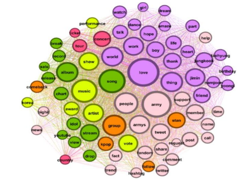
5. 소셜네트워크 분석
- 5가지 중심성 척도 degree, betweenness, closeness, eigenvector, pagerank를 통해 단어들의 연관성과 빈도 수 등을 통해 어떤 단어가 중요하게 나오는지 알아봅니다.
- Gephi를 이용하여 시각화
|
1
2
3
4
5
6
7
8
9
10
11
12
13
14
15
16
17
18
19
20
21
22
23
24
25
26
27
28
29
30
31
32
33
34
35
36
37
38
39
40
41
42
43
44
45
46
47
48
49
50
51
52
53
54
55
56
57
58
59
60
61
62
63
64
65
66
67
68
69
70
71
72
73
74
75
76
77
|
import matplotlib.pyplot as plt
count = {} # 동시출현 빈도 저장 dict
for tokens in texts:
stopped_tokens = [i for i in list(set(tokens)) ]
for i,a in enumerate(stopped_tokens):
for b in stopped_tokens[i+1:]:
if a>b:
count[b,a] = count.get((b,a),0) + 1
else:
count[a,b] = count.get((a,b),0) + 1
df = pd.DataFrame.from_dict(count, orient='index')
list1=[]
for i in range(len(df)):
list1.append([df.index[i][0], df.index[i][1], df[0][i]])
df2 = pd.DataFrame(list1, columns=['term1','term2','freq'])
df2 = df2.sort_values(by=['freq'], ascending=False) # freq 기준으로 내림차순 정렬
df2 = df2.reset_index(drop=True)
import networkx as nx
import operator
G_centrality = nx.Graph() #중심성 척도 계싼을 위한 G
for ind in range(len(np.where(df3['freq']>=3)[0])): #빈도수 3이상인 단어쌍에 대해서만 edge 표현
G_centrality.add_edge(df3['term1'][ind],df3['term2'][ind],weight=int(df3['freq'][ind]))
dgr = nx.degree_centrality(G_centrality) #연결 중심성
btw = nx.betweenness_centrality(G_centrality) #매개 중심성
cls = nx.closeness_centrality(G_centrality) #근접 중심성
egv = nx.eigenvector_centrality(G_centrality) #고유벡터 중심성
pgr = nx.pagerank(G_centrality) # 페이지랭크
#중심성 큰 순서대로 저장
sorted_dgr = sorted(dgr.items(), key= operator.itemgetter(1), reverse = True)
sorted_btw = sorted(btw.items(), key= operator.itemgetter(1), reverse = True)
sorted_cls = sorted(cls.items(), key= operator.itemgetter(1), reverse = True)
sorted_egv = sorted(egv.items(), key= operator.itemgetter(1), reverse = True)
sorted_pgr = sorted(pgr.items(), key= operator.itemgetter(1), reverse = True)
G=nx.Graph() #단어 네트워크를 그려줄 Graph선언 (저는 Gephi를 사용해서 그렸습니다.)
#페이지 랭크에 따라 두 노드 사이의 연관성을 결정 (연관성)
#연결 중심성으로 계산한 척도에 따라 노드의 크기가 결정 (빈도 수)
for i in range(len(sorted_pgr)):
G.add_node(sorted_pgr[i][0], nodesize = sorted_dgr[i][1])
for ind in range(len(np.where(df3['freq']>=3)[0])):
G.add_weighted_edges_from([(df3['term1'][ind],df3['term2'][ind],int(df3['freq'][ind]))])
# 노드 크기 조정
sizes = [G.nodes[node]['nodesize']*500 for node in G]
options = {
'edge_color':'#FFDEA2',
'width':1,
'with_labels':True,
'font_weight':'regular'
}
nx.draw(G, node_size=sizes, pos=nx.spring_layout(G, k=3.5, iterations=100), **options)
ax = plt.gca()
ax.collections[0].set_edgecolor("#555555")
plt.show()
nx.write_gexf(G, 'BTS_17.gexf') #Gephi에 사용할 수 있는 file로 저장
|
cs |
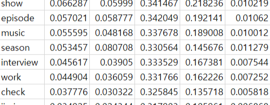
- 각 중심성 척도 값을 저장
|
1
2
3
4
5
6
7
8
9
10
11
12
13
14
15
|
aa = pd.DataFrame(sorted_dgr)
aa.columns=['keyword','degree']
aa1 = pd.DataFrame(sorted_btw)
aa1.columns=['keyword','betweenness']
aa2 = pd.DataFrame(sorted_cls)
aa2.columns=['keyword','closeness']
aa3 = pd.DataFrame(sorted_egv)
aa3.columns=['keyword','eigenvector']
aa4 = pd.DataFrame(sorted_pgr)
aa4.columns=['keyword','pagerank']
m1 = pd.merge(aa,aa1, how='outer',on='keyword')
m2 = pd.merge(m1,aa2, how='outer',on='keyword')
m3 = pd.merge(m2,aa3, how='outer',on='keyword')
m4 = pd.merge(m3,aa4, how='outer',on='keyword')
m4.to_csv('BTS_17_C.csv') # 이 부분은 노가다로 저장하는것 보다 더 좋은 방법이 있을 것.
|
cs |
6. 결과 해석


7. 결론 및 한계점


'Data 분석' 카테고리의 다른 글
| [A/B Test] E-commerce conversion ab test data (0) | 2024.06.27 |
|---|---|
| News Map 만들기 - PyQt5 (0) | 2021.09.09 |
| CNN을 통한 구름 분류 (0) | 2021.08.25 |
| 휴대폰 사진 정보를 활용한 날씨확인 (0) | 2021.08.25 |


